The radix-2 Cooley-Tukey FFT Algorithm with Decimation in Time

EDIT May 29th 2009: The code presented in this post has a major bug in the calculation of inverse DFTs using the FFT algorithm. Some explanation can be found here, and fixed code can be found here.

Once the DFT has been introduced, it is time to start computing it efficiently. Focusing on the direct transform,

if the size of the input is even, we can write N = 2·M and it is possible to split the N element summation in the previous formula into two M element ones, one over n = 2·m, another over n = 2·m + 1. By doing so, after some cancellations in the exponents we arrive at

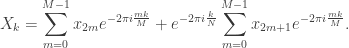
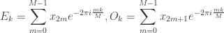
There’s something very promising here: each of the two summations are very close to being the expression of a DFT of half the size of the original. The only thing preventing them from fully being so is the fact that k runs from 0 to N-1, rather than up to M-1 only. To get around this, we will consider two different cases: k < M and k ≥ M. The first trivially produces a pair of half sized DFTs, which we will term E_k and O_k, owing to one running over the even indexes, the other over the odd ones:

.

As for the case k ≥ M, we may as well write it out as k = M + k’. And if we plug this value into the original formula, work a little with the algebra, and then undo the variable change, i.e. plug k’ = M – k back in, we arrive at the following combined formula,

.

The cool thing about this decomposition is that we have turned our N element DFT into two N/2 DFTs, plus some overhead composing the results, which includes calculating twiddle factors, i.e. the complex exponential multiplying the O’s in the last formula. Given the quadratic nature of the time required to calculate the DFT, this amounts to cutting the time in half. And the best part is that we need not stop after one such decomposition: if the original size is a power of two, we can keep doing the same trick recursively until we reach a DFT of only two elements, for which we already have produced explicit formulas. A similar approach can be used for the inverse DFT, the details are built into the following code…

from __future__ import division
import math
import time

def fft_CT(x, inverse = False, verbose = False) :
    """
    Computes the DFT of x using Cooley-Tukey's FFT algorithm.
    """
    t = time.clock()
    N = len(x)
    inv = -1 if not inverse else 1
    if N % 2 :
        return dft(x, inverse, False)
    x_e = x[::2]
    x_o  = x[1::2]
    X_e = fft_CT(x_e, inverse, False)
    X_o  = fft_CT(x_o, inverse, False)
    X = []
    M = N // 2
    for k in range(M) :
        X += [X_e[k] + X_o[k] * math.e ** (inv * 2j * math.pi * k / N)]
    for k in range(M,N) :
        X += [X_e[k-M] - X_o[k-M] * math.e ** (inv * 2j * math.pi * (k-M) / N)]
    if inverse :
        X = [j/2 for j in X]
    t = time.clock() - t
    if verbose :
        print "Computed","an inverse" if inverse else "a","CT FFT of size",N,
        print "in",t,"sec."
    return X

The speed gain with this approach, restricted for now to power of two sizes, are tremendous even for moderately large input sizes. Mostly so due to the fact the new algorithm scales as N log N. For instance, a 2²⁰ (~10⁶) item input can be processed with the FFT approach in a couple of minutes, while the projected duration using the naive DFT will be more like a couple of weeks…

Twiddle Factors Again
While it may not be immediately obvious, the previous code is generously wasting resources by calculating over and over again the same twiddle factors. Imagine, for instance, a 1024 element DFT computed using this algorithm. At some point in the recursion the original DFT will have been exploded into 64 DFTs of 16 elements each. Each of this 64 DFTs must then be composed with the exact same 8 different twiddle factors, but right now they are being calculated from scratch each of the 64 times. Furthermore, half of this 8 different twiddle factors are the same that where needed to compose the 128 DFTs of 8 elements into the 64 DFTs of 16 elements… Summing it all up, to compute a FFT of size 2ⁿ, which requires the calculation of 2^n-1 different twiddle factors, we are calculating as many as n·2^n-1 of them.

We can easily work around this by precalculating them first, and then passing the list to other functions. For instance as follows…

def fft_CT_twiddles(x, inverse = False, verbose = False, twiddles = None) :
    """
    Computes the DFT of x using Cooley-Tukey's FFT algorithm. Twiddle factors
    are precalculated in the first function call, then passed down recursively.
    """
    t = time.clock()
    N = len(x)
    inv = -1 if not inverse else 1
    if N % 2 :
        return dft(x, inverse, False)
    M = N // 2
    if not twiddles :
        twiddles = [math.e**(inv*2j*math.pi*k/N) for k in xrange(M)]+[N]
    x_e = x[::2]
    x_o  = x[1::2]
    X_e = fft_CT_twiddles(x_e, inverse, False, twiddles)
    X_o  = fft_CT_twiddles(x_o, inverse, False, twiddles)
    X = []
    for k in range(M) :
        X += [X_e[k] + X_o[k] * twiddles[k * twiddles[-1] // N]]
    for k in range(M,N) :
        X += [X_e[k-M] - X_o[k-M] * twiddles[(k - M) * twiddles[-1] // N]]
    if inverse :
        X = [j/2 for j in X]
    t = time.clock() - t
    if verbose :
        print "Computed","an inverse" if inverse else "a","CT FFT of size",N,
        print "in",t,"sec."
    return X

This additional optimization does not improve the time scaling of the algorithm, but reduces the calculation time to about two thirds of the original one.