The Cooley-Tukey FFT Algorithm for General Factorizations

(All code examples in the post have been included in the nrp_base.py module, which can be downloaded from this repository.)

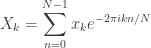
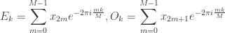
As presented in the previous post, Cooley-Tukey’s FFT algorithm has a clear limitation: it can only be used to speed the calculation of DFTs of a size that is a power of two. It isn’t hard, though, to extend the same idea to a more general factorization of the input signal size. We start again from the formula that defines the DFT,

Say that N = P·Q. Following the previous approach, we could try to split the calculation of the DFT into Q DFTs of size P, by rewriting it as

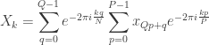
where n = Q·p + q. We are again faced with the same issue to turn the inner summation into a proper DFT: while p ranges from 0 to P-1, k goes all the way up to N-1. To get around this, we can make k = P·r + s, and replacing in the previous formula we get

where the inner summation has been reduced to a standard DFT of size P. Furthermore, the splitting of the first exponential in two factors unveils that the outer summation is also a standard DFT, this one of size Q, of the product of the DFT of size P by twiddle factors.

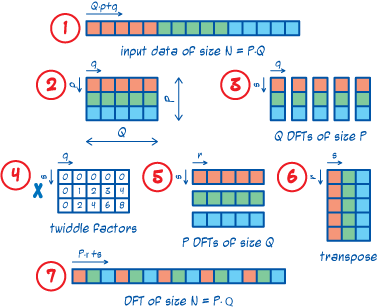
The subscripts in the above formula can get confusing to follow, so take note that q and r go from 0 to Q-1, while p and s go from 0 to P-1. Therefore the computation of the size N DFT has effectively been split into the computation of Q DFTs of size P, followed by twiddle factor multiplication, and then by P DFTs of size Q. It may be helpful to picture the linear array of input data as a PxQ matirx stored in row-major order. Then the Q DFTs of size P are performed on the columns of this matrix, and the P DFTs of size Q on the rows. Note though that the output has to be rearranged, in what would be equivalent to a matrix transposition, before getting to the final answer. As an example, the following picture illustrates the process on an input of size 15.

Planning a Generalized Cooley-Tukey FFT

Disregarding the multiplication by twiddle factors and the matrix transpositions, the algorithm turns a calculation which requires a time proportional to N² = P²Q², into one which requires a time proportional to P·Q·(P+Q). This very simplistic complexity analysis suggests that the factoring of the size of the original signal into two multiplicative factors isn’t arbitrary, and will affect the performance of the algorithm. And in principle a split into two similarly sized factors, P ~ Q ~ √N should, although often doesn’t, outperform any other approach.

In many practical applications a small P or Q is used, which is then called the radix. If the smaller DFT is in the outer loop. i.e. if Q is the radix, the scheme is termed decimation in time (DIT), while if it is in the inner loop, i.e. if P is the radix, we have decimation in frequency (DIF), which explains the long name of the simplest Cooley-Tukey algorithm described earlier.

The splitting of the input size, N, into the two multiplicative factors, P and Q, can be done in d(N) – 2 different ways, where d(N) is the divisor function, i.e. the number of divisors of N. If we use the same algorithm recursively, the possible paths to the solution can grow very fast, and determining the optimal one is anything but easy. It is in any case a point where we don’t want to make excessive assumptions, and which should be left sufficiently open for user experimentation. So I’ve decided to copy FFTW‘s approach: the first step to peform a FFT is to plan it. In our case, a plan is a data structure which is similar to a tree, holding the information of the factorizations chosen, the function that should be called to perform the next step, and references to those next steps. The following picture sketches two possible plans for a DFT of size 210 = 2·3·5·7.

In line with the image, I have coded a planning function that gives two choices to the user:

• decimation in time (dit=True) vs. decimation in frequency (dif=True)
• minimum possible radix (min_rad=True) vs. maximum possible radix (max_rad=True)

Note that the standard radix 2 with decimation in time plan would result from setting dit=True and min_rad=True when the input size is a power of two, and that it would be the default behavior of this planner.

@nrp_base.performance_timer
def plan_fft(x, **kwargs) :
    """
    Returns an FFT plan for x.

    The plan uses direct DFT for prime sizes, and the generalized CT algorithm
    with either maximum or minimum radix for others.

    Keyword Arguments
     dif     -- If True, will use decimation in frequency. Default is False.
     dit     -- If True, will use decimation in time. Overrides dif. Default
                is True.
     max_rad -- If True, will use tje largest possible radix. Default is False.
     min_rad -- If True, will use smallest possible radix. Overrides max_rad.
                Default is True.
               
    """
    dif = kwargs.pop('dif', None)
    dit = kwargs.pop('dit', None)
    max_rad = kwargs.pop('max_rad', None)
    min_rad = kwargs.pop('min_rad', None)
    
    if dif is None and dit is None :
        dif = False
        dit = True
    elif dit is None :
        dit = not dif
    else :
        dif = not dit

    if max_rad is None and min_rad is None :
        max_rad = False
        min_rad = True
    elif min_rad is None :
        min_rad = not max_rad
    else :
        max_rad = not min_rad
        
    N = len(x)
    plan = []

    if min_rad :
        fct = sorted(nrp_numth.naive_factorization(N))
        NN = N
        ptr = plan
        for f in fct :
            NN //= f
            P = [f, dft, None]
            Q = [NN, fft_CT, []]
            if dit :
                ptr += [Q, P]
            else :
                ptr += [P, Q]
            if NN == fct[-1] :
                Q[1:3] = [dft, None]
                break
            else :
                ptr = Q[2]
    else :
        items ={}
        def follow_tree(plan, N, fct, **kwargs) :
            if fct is None:
                fct = nrp_numth.naive_factorization(N)
            divs = sorted(nrp_numth.divisors(fct))
            val_P = divs[(len(divs) - 1) // 2]
            P = [val_P]
            if val_P in items :
                P = items[val_P]
            else :
                fct_P = nrp_numth.naive_factorization(val_P)
                if len(fct_P) > 1 :
                    P += [fft_CT, []]
                    follow_tree(P[2], val_P, fct_P, dit = dit)
                else :
                    P +=[dft, None]
                items[val_P] = P
            val_Q = N // val_P
            Q = [val_Q]
            if val_Q in items :
                Q = items[val_Q]
            else :
                fct_Q = nrp_numth.naive_factorization(val_Q)
                if len(fct_Q) > 1 :
                    Q += [fft_CT, []]
                    follow_tree(Q[2], val_Q, fct_Q, dit = dit)
                else :
                    Q +=[dft, None]
                items[val_Q] = Q
            if dit :
                plan += [Q, P]
            else :
                plan += [P, Q]

        follow_tree(plan, N, None, dit = dit)

    return plan

While the planner can probably be further optimized, especially for max_rad=True, with all the repeated factorizations, this shouldn’t be the critical part of the DFT calculation. Specially so since the plan can be calculated in advance, and reused for all inputs of the same size.

Twiddle Factors Reloaded

As already discussed in previous posts, one of the simplest ways of trimming down the computation time is to store the twiddle factors, which are almost certain to show up again, and reuse them whenever possible, rather than going through complex exponentiations over and over again. There is a slight difference though with regard to the radix 2 case. There, when computing a size N FFT, the twiddle factors that intervened in the calculations where all those with numerators in the exponent (apart from the ±2·π·i) ranging from 0 to N/2 – 1, inclusive. If N is split as P·Q, rather than as 2·N/2, then the largest numerator that will appear will be (P-1)·(Q-1), which is definitely larger than N/2, but not all of the items up to that value will be required, with many of them missing.

Take for instance a DFT of size 512. If we go for the radix 2 FFT, we will in total use 256 different twiddle factors, ranging from 0 to 255. If rather than that we go for a max_rad=True approach, the first split will be 512 = 16·32, and so the largest twiddle factor will have numerator 15·31 = 465. But with all the intermediate twiddle factors not showing up in the calculation, overall only 217 different ones are needed.

It is also interesting to note that the same twiddle factors that are used in the FFTs, may appear in the DFTs of the leaves of the planning tree. So it is worth modifying the current dft function, so that it can accept precalculated twiddles. Because the twiddle factors sequence will have gaps, a list is no longer the most convenient data structure to hold these values, a dictionary being a better fit for the job. Combining all of these ideas, we can rewrite our function as

@nrp_base.performance_timer
def dft(x, **kwargs) :
    """
    Computes the (inverse) discrete Fourier transform naively.

    Arguments
     x         - Te list of values to transform

    Keyword Arguments
     inverse   - True to compute an inverse transform. Default is False.
     normalize - True to normalize inverse transforms. Default is same as
                 inverse.
     twiddles  - Dictionary of twiddle factors to be used by function, used
                 for compatibility as last step for FFT functions, don't set
                 manually!!!

    """
    inverse = kwargs.pop('inverse',False)
    normalize = kwargs.pop('normalize',inverse)
    N = len(x)
    inv = -1 if not inverse else 1
    twiddles = kwargs.pop('twiddles', {'first_N' : N, 0 : 1})
    NN = twiddles['first_N']
    X =[0] * N
    for k in xrange(N) :
        for n in xrange(0,N) :
            index = (n * k * NN // N) % NN
            twid= twiddles.setdefault(index,
                                      math.e**(inv*2j*math.pi*index/NN))
            X[k] += x[n] * twid
        if inverse and normalize :
             X[k] /= NN
    return X

Note also the changes to the user interface, with the addition of the normalize keyword argument. This has been introduced to correct a notorious bug in the inverse DFT calculations for the radix 2 FFT algorithm. The changes are implemented and can be checked in the module nrp_dsp.py, although they are very similar in nature to what will shortly be presented for the generalized factorization FFT.

Putting it all Together

We now have most of the building blocks to put together a FFT function using Cooley-Tukey’s algorithm for general factorizations, a possible realization of which follows:

@nrp_base.performance_timer
def fft_CT(x, plan,**kwargs) :
    """
    Computes the (inverse) DFT using Cooley-Tukey's generalized algorithm.
    
    Arguments
     x        - The list of values to transform.
     plan     - A plan data structure for FFT execution.

    Keyword Arguments
     inverse  - if True, computes an inverse FFT. Default is False.
     twiddles - dictionary of twiddle factors to be used by function, used
                for ptimization during recursion, don't set manually!!!
                                
    """
    inverse = kwargs.pop('inverse', False)
    inv = 1 if inverse else -1
    N = len(x)
    twiddles = kwargs.pop('twiddles', {'first_N' : N, 0 : 1})
    NN = twiddles['first_N']
    X = [0] * N
    P = plan[0]
    Q = plan[1]
    # do inner FFT
    for q in xrange(Q[0]) :
        X[q::Q[0]] = P[1](x[q::Q[0]], plan=P[2], twiddles=twiddles,
                          inverse=inverse,normalize=False)
    # multiply by twiddles
    for q in xrange(Q[0]) :
        for s in xrange(P[0]) :
            index = q * s * NN // N
            
            mult = twiddles.setdefault(index,
                                       math.e**(inv*2j*math.pi*index/NN))
            X[Q[0]*s+q] *= mult
    # do outer FFT
    for s in xrange(P[0]) :
        X[Q[0]*s:Q[0]*(s+1)] = Q[1](X[Q[0]*s:Q[0]*(s+1)],plan=Q[2],
                                    twiddles=twiddles,inverse=inverse,
                                    normalize=False)
    # transpose matrix
    ret = [0] * N
    for s in xrange(P[0]) :
        ret[s::P[0]] = X[s*Q[0]:(s+1)*Q[0]]
    if inverse and N == NN : # normalize inverse only in first call
        ret = [val / N for val in ret]
    return ret

For power of two sizes, this algorithm is noticeably slower, by a factor of more than 2 depending on the input size, than the hardcoded radix 2 prior version. This is mostly due to the time spent doing matrix inversion in the last step. Also due to the matrix inversion, minimum radix plans usually outperform maximum radix ones, despite the benefits in FFT and twiddle factor computations the latter present over the former. Of course none of this matters if the input size presents several prime factors other than two, in which case the new algorithm clearly outperforms the radix 2 version, which is then close to the DFT version. Still, it is worth noting for later optimizations that matrix inversion should be done in a more efficient fashion.

The radix-2 Cooley-Tukey FFT Algorithm with Decimation in Time

EDIT May 29th 2009: The code presented in this post has a major bug in the calculation of inverse DFTs using the FFT algorithm. Some explanation can be found here, and fixed code can be found here.

Once the DFT has been introduced, it is time to start computing it efficiently. Focusing on the direct transform,

if the size of the input is even, we can write N = 2·M and it is possible to split the N element summation in the previous formula into two M element ones, one over n = 2·m, another over n = 2·m + 1. By doing so, after some cancellations in the exponents we arrive at

There’s something very promising here: each of the two summations are very close to being the expression of a DFT of half the size of the original. The only thing preventing them from fully being so is the fact that k runs from 0 to N-1, rather than up to M-1 only. To get around this, we will consider two different cases: k < M and k ≥ M. The first trivially produces a pair of half sized DFTs, which we will term E_k and O_k, owing to one running over the even indexes, the other over the odd ones:

.

As for the case k ≥ M, we may as well write it out as k = M + k’. And if we plug this value into the original formula, work a little with the algebra, and then undo the variable change, i.e. plug k’ = M – k back in, we arrive at the following combined formula,

.

The cool thing about this decomposition is that we have turned our N element DFT into two N/2 DFTs, plus some overhead composing the results, which includes calculating twiddle factors, i.e. the complex exponential multiplying the O’s in the last formula. Given the quadratic nature of the time required to calculate the DFT, this amounts to cutting the time in half. And the best part is that we need not stop after one such decomposition: if the original size is a power of two, we can keep doing the same trick recursively until we reach a DFT of only two elements, for which we already have produced explicit formulas. A similar approach can be used for the inverse DFT, the details are built into the following code…

from __future__ import division
import math
import time

def fft_CT(x, inverse = False, verbose = False) :
    """
    Computes the DFT of x using Cooley-Tukey's FFT algorithm.
    """
    t = time.clock()
    N = len(x)
    inv = -1 if not inverse else 1
    if N % 2 :
        return dft(x, inverse, False)
    x_e = x[::2]
    x_o  = x[1::2]
    X_e = fft_CT(x_e, inverse, False)
    X_o  = fft_CT(x_o, inverse, False)
    X = []
    M = N // 2
    for k in range(M) :
        X += [X_e[k] + X_o[k] * math.e ** (inv * 2j * math.pi * k / N)]
    for k in range(M,N) :
        X += [X_e[k-M] - X_o[k-M] * math.e ** (inv * 2j * math.pi * (k-M) / N)]
    if inverse :
        X = [j/2 for j in X]
    t = time.clock() - t
    if verbose :
        print "Computed","an inverse" if inverse else "a","CT FFT of size",N,
        print "in",t,"sec."
    return X

The speed gain with this approach, restricted for now to power of two sizes, are tremendous even for moderately large input sizes. Mostly so due to the fact the new algorithm scales as N log N. For instance, a 2²⁰ (~10⁶) item input can be processed with the FFT approach in a couple of minutes, while the projected duration using the naive DFT will be more like a couple of weeks…

Twiddle Factors Again
While it may not be immediately obvious, the previous code is generously wasting resources by calculating over and over again the same twiddle factors. Imagine, for instance, a 1024 element DFT computed using this algorithm. At some point in the recursion the original DFT will have been exploded into 64 DFTs of 16 elements each. Each of this 64 DFTs must then be composed with the exact same 8 different twiddle factors, but right now they are being calculated from scratch each of the 64 times. Furthermore, half of this 8 different twiddle factors are the same that where needed to compose the 128 DFTs of 8 elements into the 64 DFTs of 16 elements… Summing it all up, to compute a FFT of size 2ⁿ, which requires the calculation of 2^n-1 different twiddle factors, we are calculating as many as n·2^n-1 of them.

We can easily work around this by precalculating them first, and then passing the list to other functions. For instance as follows…

def fft_CT_twiddles(x, inverse = False, verbose = False, twiddles = None) :
    """
    Computes the DFT of x using Cooley-Tukey's FFT algorithm. Twiddle factors
    are precalculated in the first function call, then passed down recursively.
    """
    t = time.clock()
    N = len(x)
    inv = -1 if not inverse else 1
    if N % 2 :
        return dft(x, inverse, False)
    M = N // 2
    if not twiddles :
        twiddles = [math.e**(inv*2j*math.pi*k/N) for k in xrange(M)]+[N]
    x_e = x[::2]
    x_o  = x[1::2]
    X_e = fft_CT_twiddles(x_e, inverse, False, twiddles)
    X_o  = fft_CT_twiddles(x_o, inverse, False, twiddles)
    X = []
    for k in range(M) :
        X += [X_e[k] + X_o[k] * twiddles[k * twiddles[-1] // N]]
    for k in range(M,N) :
        X += [X_e[k-M] - X_o[k-M] * twiddles[(k - M) * twiddles[-1] // N]]
    if inverse :
        X = [j/2 for j in X]
    t = time.clock() - t
    if verbose :
        print "Computed","an inverse" if inverse else "a","CT FFT of size",N,
        print "in",t,"sec."
    return X

This additional optimization does not improve the time scaling of the algorithm, but reduces the calculation time to about two thirds of the original one.